
논문을 선정한 이유
- 이미지/영상처리를 수행하면서 가장 자주 사용하는 스킬이 object detection과 segmentation
- UNet은 이미지 segmentation에서 지금까지도 basemodel로 사용하고 있는 기본 모델
- Convolution 기반으로 모델 아키텍쳐가 이해하기 쉬움
논문 읽기
Abstract

이 논문에서는 모델 네트워크와 모델 훈련 전략을 제시한다. 여기서 제시하는 전략은 사용 가능한 annotation 샘플을 더 효율적으로 사용하기 위해서 데이터증강을 강하게 사용하는 것을 말한다.
이를 위해서 모델 아키텍처는 contracting path와 expanding path가 대칭을 이루고 있으며, contracting path에서는 특정 context를 캡쳐하는 역할을 하고 expanding path에서는 이 캡쳐본을 정확한 위치에 적용하는 역할을 한다. 이 말은 밑에 UNet의 구조를 그림으로 보면 더 잘 이해할 수 있다.
Introduction
<요약>
- train 데이터가 적은 경우를 대비해서 이미지증강을 적극 활용
- 모델은 contracting path와 expanding path로 이루어짐
- 고해상도 유지를 위해 contracting path에서 사용했던 feature를 expanding path에서 추가
- expanding path에서는 max pooling대신 up sampling convolution 사용

그동안의 이미지 모델은 훈련하는데 오랜 시간이 걸리기도 했고, 일반적으로 단일 label 분류 작업에 사용되었다. 하지만 의학분야에서는 label이 이미지단위가 아닌 픽셀단위에 할당되어야하는 경우가 많았다. 따라서 UNet에서는 각 필셀의 label을 예측하는 하는 것을 기반으로, fully convolutional network의 pooling 단계 대신에 expanding path에서 up sampling 연산을 수행하여 네트워크를 보완하고, contracting path에서 가져온 고해상도 feature를 더해 localize 해준다.
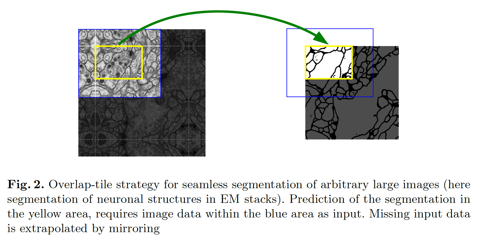
UNet에서는 완전히 연결된 레이어를 사용하는 것이 아니라 각 컨볼루션의 유효한 부분만 사용하여 Fig2와 같이 오버랩 타일 전략으로 segmentation을 예측한다. 오버랩 타일 전략은 GPU 상황에 따른 해상도 제한 없이 큰 이미지에도 모델을 적용하기 위해서 사용된다.
Overlap tile은 위 그림에서 input은 파란색 테투리 범위만큼 들어가지만 output은 노란색만큼만 나오게 하고, 다음단계에서는 파란색 부분이 겹치게끔 input을 잡고 그보다 작게 output이 나오게 하는 방법으로 겹치는 부분이 존재하도록 이미지를 자르고 segmentation하는 방법이다.
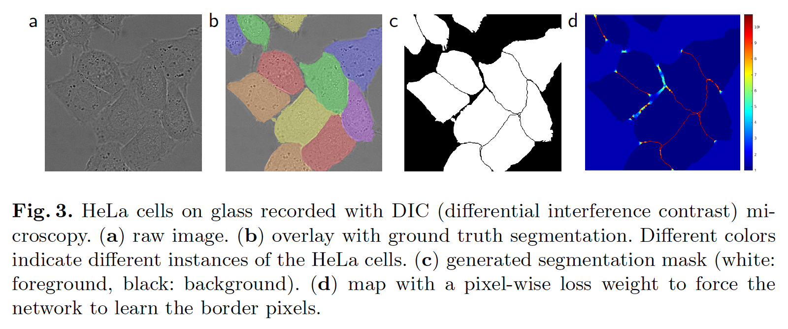
Fig3.과 같이 같은 label을 가진 세포 등의 segmentation을 수행하는 경우 세포 사이의 배경 레이블이 작을수록 배경 레이블의 손실함수가 큰 가중치를 얻게되는 가중 손실 사용을 제안한다. 생물 의학의 segmentation 문제에 적용하기에 좋은 방법이다.
Network Architecture
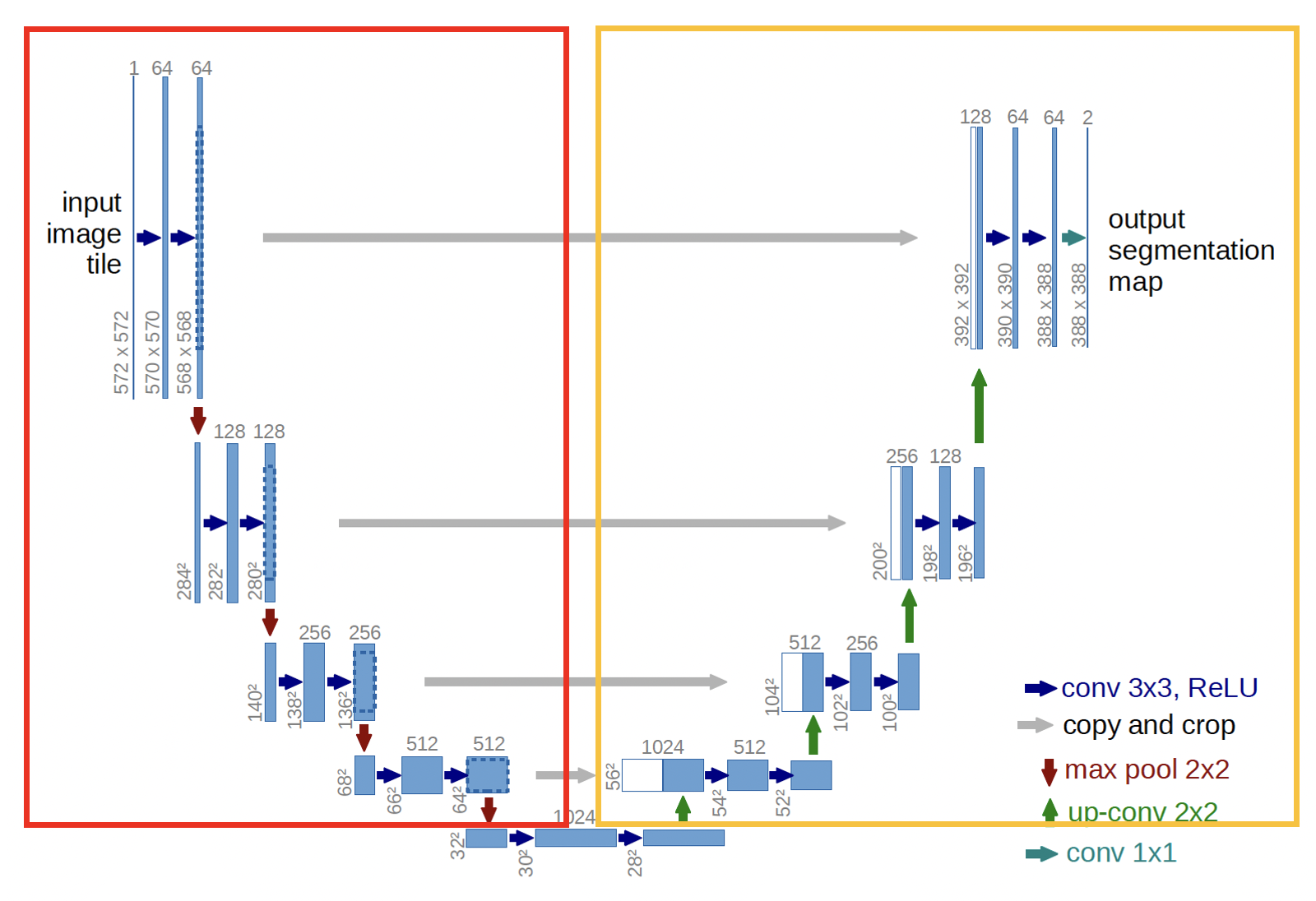
위에 있는 Fig1이 네트워크 구조다. 빨간색 박스 부분이 contract path로 일반적인 컨볼루션 아키텍쳐를 따라간다.input image channeldl 1에서 1024까지 증가한다. 각 stage의 마지막 layer feature를 변수로 넣어서 expanding path의 동일한 stage에 전달한다. 노란색 박스 부분이 expanding path로 channel이 1024였던 데이터를 output segmentation에 맞춰서 줄여준다. 맨 밑의 단계는 일부러 박스에 포함을 안시켰는데 contract path에서 expanding path로 전환되는 전환구간이라고 생각하면 된다.
output segmentation map에 over-lap tile을 수행하기 위해서 2x2 max pooling을 해줘야 한다. 이 때, max pooling에 들어가는 x, y가 모두 짝수가 되도록 input tile size를 생각해줘야 한다.
Training
input image와 그에 대응하는 segmentaion map은 확률적 경사하강법을 학습에 사용한다.
padding을 하지 않은 convolution이 있기 때문에 output image는 input image보다 일정한 width만큼 작다.
오버헤드를 최소화하고 GPU 메모리를 최대한 활용하기 위해 batch size를 input size보다 크게해서 하나의 배치에 하나의 이미지를 만든다. 이렇게 하기 위해 높은 모멘텀(0.99)를 사용한다.
Cross entropy loss function과 결합된 최종 feature map에 대해서 pixel단위로 Softmax 함수를 사용한다.
이렇게 되면 이미지 위치에 따른 pixel이 label 값을 가지게 된다.
weight initialize는 가우시안 초기화를 따랐다.
Data Augmentation
사용 가능한 train data가 많이 없을 때 데이터 증강이 필수적이다.
기본적으로 shift, rotation invariance, gray value를 사용하여 데이터를 증강했고, 추가적으로 3x3 grid에서 무작위 변위 벡터를 사용하여 부드러운 변형을 생성했다.
Experiments
3가지 segmentation task를 수행했다.
- task1 : 전자현미경으로 기록된 신경구조 segmentation (Fig2)
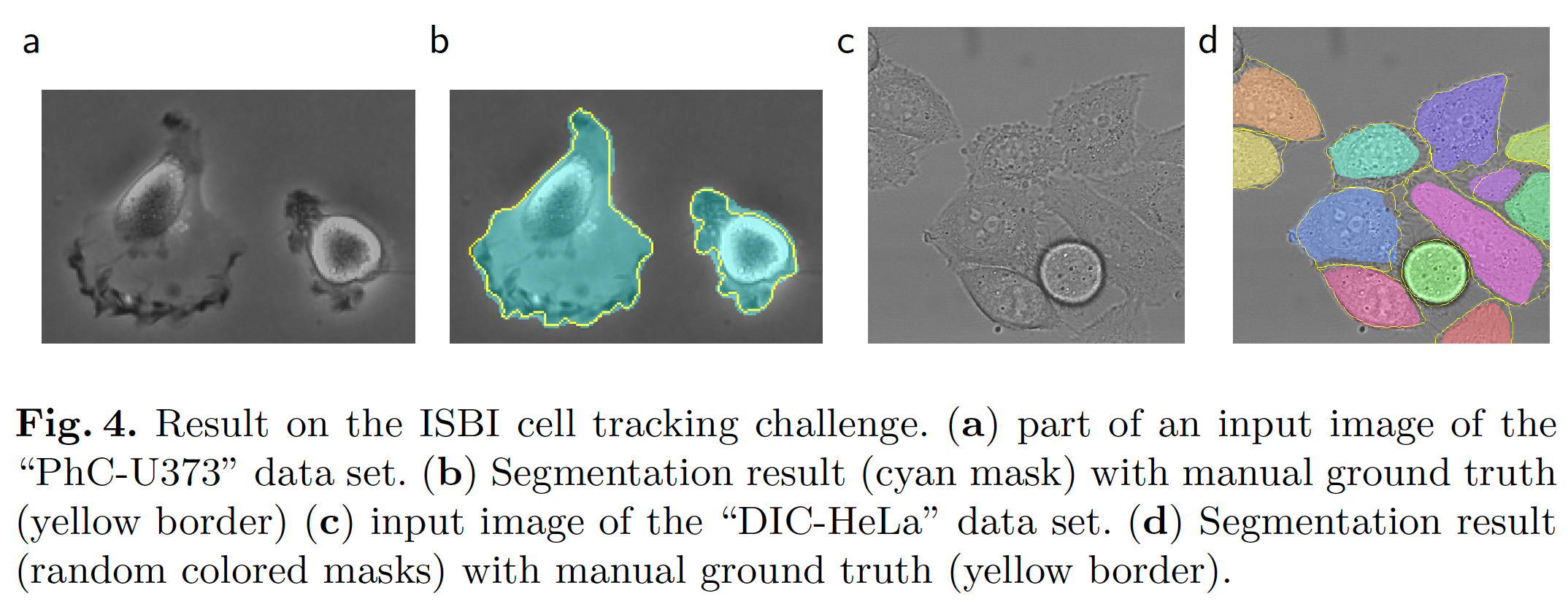
- task2 : "PhC-U373" dataset - 빛현미경으로 본 세포 이미지 segmentation (Fig4 a, b)
- task3 : "DIC-Hela" dataset - DIC 현미경으로 기록한 flat glass 위의 Hela세포 이미지 segmentation (Fig4 c, d)
task1의 경우 Warping Error, Rand Error, Pixel Error를 평가지표로 사용하여 매우 낮은 오류율을 보였다.
task2, 3의 경우 2015년 ISBI cell tracking challenge에서 IOU 평가 결과 가장 높은 성능을 보였다.
Conclusion
UNet은 매우 다른 Bio 분야에서 수행하는 segmentation에도 우수한 성능을 보인다.
부드러운 변형을 통한 데이터 증강 덕분에 annotation이 된 이미지가 많이 없어도 학습이 가능했고,
NVidia Titan GPU(6GB)를 이용한 학습시간이 10시간밖에 걸리지 않았다.
UNet 아키텍쳐는 더 많은 작업에 쉽게 적용될 수 있다고 확신한다.
논문리뷰
저자가 뭘 해내고 싶어했는가?
Bio분야에서 동일한 label을 가지지만 서로 붙어있는 경우에도 segmentation을 잘 수행할 수 있는 방법을 찾음
이 연구의 접근에서 중요한 요소는 무엇인가?
배경의 손실함수에 가중치를 두어서 그 범위가 작을수록 더 잘 구분할 수 있도록 한 점
이전에 사용한 feature를 expanding path에 적용하여 고해상도 유지와 더불어 segmentation을 잘 수행하도록 한 점
2x2 max-pooling을 위한 input size를 짝수로 맞춰줘야하는 점
논문을 보고 느낀점?
convolution을 기본으로 이전의 feature를 가져온다는 아이디어는 매우 좋았다.
이 분야에 오래 있는 사람이라면 한번쯤 생각해볼만 한 아이디어인데 그걸 코드로 완성시켰다는 점이 대단하다.
어떤 프로젝트에 적용할 수 있는가?
label 구별이 필요한 대상들이 뭉쳐있는 이미지인 경우 segmentation을 진행할 때 그 경계선을 잘 구분할 수 있을듯
일반사진보다 배경이 단색으로 통일되어있는 경우 (bio cell 등) 더 잘 구별할 수 있을 것 같음
추가적으로 공부해야할 것 또는 참고하고 싶은 다른 레퍼런스에는 어떤 것이 있는가?
또 다른 기법인 yolo를 공부해보고싶다.
UNet 코드 구현
각 layer 이름을 path이름stage넘버_layer넘버로 작성했다.
여기서 contract path는 encoder인 enc로, expanding path는 decoder인 dec로 표기했다.
예를들어 contract path의 첫번재 stage의 첫번째 layer라면 enc1_1라고 표시했다.
decoder부분의 경우에는 encoder와 pair를 맞추기 위해 stage와 layer를 거꾸로 쌓았다.
코드를 한줄씩 보면 잘 이해가 될꺼라고 생각한다.
class UNet(nn.Module):
    def __init__(self):
        super(UNet, self).__init__()

        # conv 3x3, batch normalization, relu
        def CB(in_channels, out_channels, kernel_size=3, stride=1, padding=1, bias=True):
            layers = []
            layers += [nn.Conv2d(in_channels=in_channels, out_channels=out_channels,
                                 kernel_size=kernel_size, stride=stride, padding=padding, bias=bias)]
            layers += [nn.BatchNorm2d(num_features=out_channels)]
            layers += [nn.ReLU()]

            conv_block = nn.Sequential(*layers)
            return conv_block

        # UNet Encoder
        self.enc1_1 = CB(in_channels=1, out_channels=64)
        self.enc1_2 = CB(in_channels=64, out_channels=64)
        self.pool1 = nn.MaxPool2d(kernel_size=2)

        self.enc2_1 = CB(in_channels=64, out_channels=128)
        self.enc2_2 = CB(in_channels=128, out_channels=128)
        self.pool2 = nn.MaxPool2d(kernel_size=2)

        self.enc3_1 = CB(in_channels=128, out_channels=256)
        self.enc3_2 = CB(in_channels=256, out_channels=256)
        self.pool3 = nn.MaxPool2d(kernel_size=2)

        self.enc4_1 = CB(in_channels=256, out_channels=512)
        self.enc4_2 = CB(in_channels=512, out_channels=512)
        self.pool4 = nn.MaxPool2d(kernel_size=2)

        self.enc5_1 = CB(in_channels=512, out_channels=1024)

        # UNet Decoder
        self.dec5_1 = CB(in_channels=1024, out_channels=512)

        self.unpool4 = nn.ConvTranspose2d(in_channels=512, out_channels=512, kernel_size=2, stride=2, padding=0, bias=True)

        # in_channels = 512*2인 이유는 encoder에서 사용했던 피쳐맵을 decoder에서도 사용할 수 있도록
        # forward에서 dec와 enc을 concat해주기 때문
        self.dec4_2 = CB(in_channels=512*2, out_channels=512)
        self.dec4_1 = CB(in_channels=512, out_channels=256)

        self.unpool3 = nn.ConvTranspose2d(in_channels=256, out_channels=256, kernel_size=2, stride=2, padding=0, bias=True)
        self.dec3_2 = CB(in_channels=256*2, out_channels=256)
        self.dec3_1 = CB(in_channels=256, out_channels=128)

        self.unpool2 = nn.ConvTranspose2d(in_channels=128, out_channels=128, kernel_size=2, stride=2, padding=0, bias=True)
        self.dec2_2 = CB(in_channels=128*2, out_channels=128)
        self.dec2_1 = CB(in_channels=128, out_channels=64)

        self.unpool1 = nn.ConvTranspose2d(in_channels=64, out_channels=64, kernel_size=2, stride=2, padding=0, bias=True)
        self.dec1_2 = CB(in_channels=64*2, out_channels=64)
        self.dec1_1 = CB(in_channels=64, out_channels=64)

        self.fc = nn.Conv2d(in_channels=64, out_channels=1, kernel_size=1, stride=1, padding=0, bias=True)

    def forward(self, x):
        # Encoder
        enc1_1 = self.enc1_1(x)
        enc1_2 = self.enc1_2(enc1_1)
        pool1 = self.pool1(enc1_2)

        enc2_1 = self.enc2_1(pool1)
        enc2_2 = self.enc2_2(enc2_1)
        pool2 = self.pool2(enc2_2)

        enc3_1 = self.enc3_1(pool2)
        enc3_2 = self.enc3_2(enc3_1)
        pool3 = self.pool3(enc3_2)

        enc4_1 = self.enc4_1(pool3)
        enc4_2 = self.enc4_2(enc4_1)
        pool4 = self.pool4(enc4_2)

        enc5_1 = self.enc5_1(pool4)

        # Decoder
        dec5_1 = self.dec5_1(enc5_1)

        unpool4 = self.unpool4(dec5_1)

        # UNet 구조 중 encoder에서 사용했던 피쳐맵을 decoder에서 동일하게 사용하도록 구축
        # dim=[0:batch, 1:channel, 2:height, 3:width]
        cat4 = torch.cat((unpool4, enc4_2), dim=1)
        dec4_2 = self.dec4_2(cat4)
        dec4_1 = self.dec4_1(dec4_2)

        unpool3 = self.unpool3(dec4_1)
        cat3 = torch.cat((unpool3, enc3_2), dim=1)
        dec3_2 = self.dec3_2(cat3)
        dec3_1 = self.dec3_1(dec3_2)

        unpool2 = self.unpool2(dec3_1)
        cat2 = torch.cat((unpool2, enc2_2), dim=1)
        dec2_2 = self.dec2_2(cat2)
        dec2_1 = self.dec2_1(dec2_2)

        unpool1 = self.unpool1(dec2_1)
        cat1 = torch.cat((unpool1, enc1_2), dim=1)
        dec1_2 = self.dec1_2(cat1)
        dec1_1 = self.dec1_1(dec1_2)

        x = self.fc(dec1_1)

        return x
UNet 실습
논문에서 사용한 데이터를 쓰려고 봤더니 공식적으로 배포된 거는 더이상 구할 수 없게 되었지만,
다른 사람들이 github에 올려둔 파일을 통해서 다운받을 수 있었다.
데이터 다운로드 링크 : https://github.com/hanyoseob/youtube-cnn-002-pytorch-unet
패키지 import
import os
import numpy as np
from PIL import Image
import matplotlib.pyplot as plt

from tqdm import tqdm
import torch
import torch.nn as nn
from torch.utils.data import DataLoader
import torchvision.transforms as transforms
데이터 전처리
# 데이터 저장경로
data_dir = '/data/paper_review/unet'

name_label = 'train-labels.tif'
name_input = 'train-volume.tif'

img_label = Image.open(os.path.join(data_dir, name_label))
img_input = Image.open(os.path.join(data_dir, name_input))

ny, nx = img_label.size
nframe = img_label.n_frames

print('nx', nx)
print('ny', ny)
print('frame', nframe)
다운받은 데이터는 마치 gif파일처럼 여러개의 이미지가 순차적으로 보여지는 파일이었다.
nx x ny x nframe 형식으로 이루어져 있고, 512 x 512 이미지가 30프레임 담겨있었다.
이 30프레임을 30장의 이미지 파일로 저장한다.
# 데이터는 총 30프레임으로 구성되어 train:val:test=24:3:3
nframe_train = 24
nframe_val = 3
nframe_test = 3

# 데이터 나눠서 저장할 경로 설정
train_dir = os.path.join(data_dir, 'train')
val_dir = os.path.join(data_dir, 'val')
test_dir = os.path.join(data_dir, 'test')

# 경로 폴더 만들기
if not os.path.exists(train_dir):
    os.makedirs(train_dir)
if not os.path.exists(val_dir):
    os.makedirs(val_dir)
if not os.path.exists(test_dir):
    os.makedirs(test_dir)

# 데이터 랜덤 설정
id_frame = np.arange(nframe)
np.random.shuffle(id_frame)
print(id_frame)

# 데이터 섞어서 train 저장
offset_nframe = 0
for i in range(nframe_train):
    img_label.seek(id_frame[i + offset_nframe])
    img_input.seek(id_frame[i + offset_nframe])

    label_ = np.asarray(img_label)
    input_ = np.asarray(img_input)

    np.save(os.path.join(train_dir, f'label_{i:03d}.npy'), label_)
    np.save(os.path.join(train_dir, f'input_{i:03d}.npy'), input_)

# 데이터 섞어서 val 저장
offset_nframe += nframe_train
for i in range(nframe_val):
    img_label.seek(id_frame[i + offset_nframe])
    img_input.seek(id_frame[i + offset_nframe])

    label_ = np.asarray(img_label)
    input_ = np.asarray(img_input)

    np.save(os.path.join(val_dir, f'label_{i:03d}.npy'), label_)
    np.save(os.path.join(val_dir, f'input_{i:03d}.npy'), input_)

# 데이터 섞어서 test 저장
offset_nframe += nframe_val
for i in range(nframe_test):
    img_label.seek(id_frame[i + offset_nframe])
    img_input.seek(id_frame[i + offset_nframe])

    label_ = np.asarray(img_label)
    input_ = np.asarray(img_input)

    np.save(os.path.join(test_dir, f'label_{i:03d}.npy'), label_)
    np.save(os.path.join(test_dir, f'input_{i:03d}.npy'), input_)

# 데이터 확인
plt.subplot(121)
plt.imshow(label_, cmap='gray')
plt.title('label')

plt.subplot(122)
plt.imshow(input_, cmap='gray')
plt.title('input')

plt.show()

나누어진 데이터를 확인해보았다.
이 데이터들을 pytorch로 사용하려면 dataset, dataloader를 구성해줘야한다.
# dataset
class MyDataset(torch.utils.data.Dataset):
    def __init__(self, data_dir, transform=None):
        self.data_dir = data_dir
        self.transform = transform

        # 데이터 파일 리스트 받기
        lst_data = os.listdir(self.data_dir)

        lst_label = [f for f in lst_data if f.startswith('label')]
        lst_input = [f for f in lst_data if f.startswith('input')]

        lst_label.sort()
        lst_input.sort()

        self.lst_label = lst_label
        self.lst_input = lst_input

    def __len__(self):
        return len(self.lst_label)

    def __getitem__(self, index):
        labels = np.load(os.path.join(self.data_dir, self.lst_label[index]))
        inputs = np.load(os.path.join(self.data_dir, self.lst_input[index]))

        # normalization
        labels = labels/255.0
        inputs = inputs/255.0

        # torch는 반드시 3차원이여야하기 때문에 채널이 없는 경우 채널을 만들어주는 함수
        if labels.ndim == 2:
            labels = labels[:, :, np.newaxis]
        if inputs.ndim == 2:
            inputs = inputs[:, :, np.newaxis]

        data = {'inputs': inputs, 'labels': labels}

        if self.transform:
            data = self.transform(data)

        return data
data transpose를 수행하는데 각 함수를 데이터에 맞게 조금 수정했다.
# transform 구현
class MyToTensor(object):
    def __call__(self, data):
        inputs, labels = data['inputs'], data['labels']

        inputs = inputs.transpose((2, 0, 1)).astype(np.float32)
        labels = labels.transpose((2, 0, 1)).astype(np.float32)

        # inputs = torch.from_numpy(inputs)
        # labels = torch.from_numpy(labels)

        data = {'inputs' : torch.from_numpy(inputs), 'labels' : torch.from_numpy(labels)}

        return data

class MyNormalization(object):
    def __init__(self, mean=0.5, std=0.5):
        self.mean = mean
        self.std = std

    def __call__(self, data):
        inputs, labels = data['inputs'], data['labels']

        inputs = (inputs - self.mean) / self.std

        data = {'inputs': inputs, 'labels': labels}
        return data

class RandomFlip(object):
    def __call__(self, data):
        inputs, labels = data['inputs'], data['labels']

        # 50% 좌우 반전
        if np.random.rand() > 0.5:
            inputs = np.fliplr(inputs)
            labels = np.fliplr(labels)

        # 50% 상하 반전
        if np.random.rand() > 0.5:
            inputs = np.flipud(inputs)
            labels = np.flipud(labels)

        data = {'inputs': inputs, 'labels': labels}
        return data

# data loader가 잘 되었는지 확인
train_data = MyDataset(data_dir=os.path.join(data_dir, 'train'))
data = train_data.__getitem__(0)
inputs = data['inputs']
labels = data['labels']

print('input shape', inputs.shape)
print('label shape', labels.shape)

# 시각화
plt.subplot(121)
plt.imshow(inputs)
plt.subplot(122)
plt.imshow(labels)

모델학습
# 변수설정
lr = 0.001
batch_size = 4
n_epoch = 100

# train model 저장경로
ckpt_dir = './checkpoint'

# cpu, gpu
device = torch.device('cuda' if torch.cuda.is_available() else 'cpu')
print(device)
# transforms
train_transform = transforms.Compose([MyNormalization(),
RandomFlip(),
MyToTensor()])
test_transform = transforms.Compose([MyNormalization(),
MyToTensor()])
# Dataset
train_set = MyDataset(data_dir=os.path.join(data_dir, 'train'), transform=train_transform)
val_set = MyDataset(data_dir=os.path.join(data_dir, 'val'), transform=train_transform)
test_set = MyDataset(data_dir=os.path.join(data_dir, 'test'), transform=test_transform)
# DataLoader
train_dl = DataLoader(train_set, batch_size=batch_size, shuffle=True)
val_dl = DataLoader(val_set, batch_size=batch_size, shuffle=False)
test_dl = DataLoader(test_set, batch_size=batch_size, shuffle=False)# loss 추이 확인을 위한 변수 설정
num_data_train = len(train_set)
num_data_val = len(val_set)
num_data_test = len(test_set)
num_batch_train = np.ceil(num_data_train/batch_size)
num_batch_val = np.ceil(num_data_val/batch_size)
num_batch_test = np.ceil(num_data_test/batch_size)# 모델
model = UNet().to(device)
fn_loss = nn.BCEWithLogitsLoss().to(device)
optimizer = torch.optim.Adam(model.parameters(), lr=lr)# 그 외 함수
fn_tonumpy = lambda x: x.to('cpu').detach().numpy().transpose(0, 2, 3, 1)
fb_denorm = lambda x, meam, std: (x*std)+mean
fn_class = lambda x: 1.0*(x>0.5)
# 모델 저장
def save_model(ckpt_dir, model, optim, epoch):
if not os.path.exists(ckpt_dir):
os.makedirs(ckpt_dir)
torch.save({'model': model.state_dict(),
'optim': optim.state_dict()},
f'./{ckpt_dir}/model_{epoch:02d}.pth')# 모델학습
for epoch in range(n_epoch):
model.train()
batch_loss = []
epoch_loss = []
for batch, data in enumerate(train_dl, 1):
labels = data['labels'].to(device)
inputs = data['inputs'].to(device)
output = model(inputs)
loss = fn_loss(output, labels)
optimizer.zero_grad()
loss.backward()
optimizer.step()
# loss 계산
batch_loss += [loss.item()]
batch_loss_mean = np.mean(batch_loss)
epoch_loss += [batch_loss_mean.item()]
# 모델 val
with torch.no_grad():
model.eval()
loss_arr = []
for batch, data in enumerate(val_dl, 1):
labels = data['labels'].to(device)
inputs = data['inputs'].to(device)
output = model(inputs)
loss = fn_loss(output, labels)
loss_arr += [loss.item()]
# epoch마다 모델 저장
if epoch % 10 == 0:
print(f'Train Epoch {epoch}/{n_epoch}\tLoss {np.mean(epoch_loss):.4f}')
print(f'Valid Epoch {epoch}/{n_epoch}\tLoss {np.mean(loss_arr):.4f}')
save_model(ckpt_dir=ckpt_dir, model=model, optim=optimizer, epoch=epoch)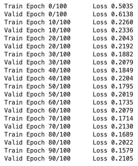
모델이 잘 학습되는 것을 볼 수 있다.
모델 test
# 모델 불러오기
def load(ckpt_dir, model, optim):
    if not os.path.exists(ckpt_dir):
        epoch = 0
        return model, optim, epoch

    ckpt_lst = os.listdir(ckpt_dir)
    ckpt_lst.sort(key=lambda f: int(''.join(filter(str.isdigit, f))))

    dict_model = torch.load(f'./{ckpt_dir}/{ckpt_lst[-1]}')

    model.load_state_dict(dict_model['model'])
    optim.load_state_dict(dict_model['optim'])
    epoch = int(ckpt_lst[-1].split('_')[1].split('.pth')[0])

    return model, optim, epoch
# 모델 테스트
st_epoch = 0
model, optimizer, st_epoch = load(ckpt_dir=ckpt_dir, model=model, optim=optimizer)
with torch.no_grad():
model.eval()
test_loss = []
for batch, data in enumerate(test_dl, 1):
labels = data['labels'].to(device)
inputs = data['inputs'].to(device)
output = model(inputs)
loss = fn_loss(output, labels)
test_loss += [loss.item()]
print(f'Test Batch {batch}/{num_batch_test}\tLoss {np.mean(test_loss)}')
프린트 해본 결과 Test Batch 1/1 Loss 0.20409727이 나와서 테스트도 잘 이루어졌다.
30프레임을 30개의 이미지로 저장한 것 중에 랜덤으로 3개의 이미지만 테스트한결과를 시각화 하면 아래와 같다.
# 테스트 결과 시각화
fig, axes = plt.subplots(output.shape[0], 3)
inputs = inputs.squeeze(1).cpu().detach().numpy()
labels = labels.squeeze(1).cpu().detach().numpy()
output = output.squeeze(1).cpu().detach().numpy()

for i in range(3):
    inputs2 = inputs[i]
    labels2 = labels[i]
    output2 = output[i]

    axes[i, 0].imshow(inputs2)
    axes[i, 0].set_title(f'inputs{i}')
    axes[i, 1].imshow(labels2)
    axes[i, 1].set_title(f'labels{i}')
    axes[i, 2].imshow(output2)
    axes[i, 2].set_title(f'output{i}')

plt.show()
눈으로 대충 봐도 inputs 대비 output이 비슷하게 그려진 것을 볼 수 있고,
labels와 비교해봐도 output이 크게 차이나지 않아서 UNet 모델의 성능을 확인할 수 있었다.
UNet 모델 역시 패키지를 사용하는 방법이 있다.
# UNet 패키지1
import torch
model = torch.hub.load('mateuszbuda/brain-segmentation-pytorch', 'unet',
    in_channels=3, out_channels=1, init_features=32, pretrained=True)

# UNet 패키지2
!pip install unet
from unet import unet

# UNet 패키지3
!pip install segmentation-models
from segmentation_models import unet
참고