
선행논문 : ResNet > MobileNet > SENet
EfficientNet에서는 MobileNet과 SENet에서 제안했던 개념이 사용되기 때문에 먼저 공부하는 것을 권장한다.
논문을 선정한 이유
- 지난번에 리뷰한 ResNet 과 함께 효율적, 범용적으로 CV 프로젝트에서 사용할 수 있을 것 같아 공부하기 위함
- ResNet 이후 한번 더 효율성을 높힌 방법론이기 때문
논문 읽기
Abstract

이 논문의 핵심 내용은 아래와 같다.
(1) 효율적인 모델 구축을 위해 depth, width, resolution을 스케일링하는 방법 제안
(2) MnasNet에서 사용하는 Conv구조인 MBConv를 이용한 EfficientNet 제안
Introduction
<요약>
- 이전 연구들에서는 모델 성능을 높이기 위해 depth, width, image size 중 하나만 scaling 함
- depth, width, image size 사이의 관계를 수식으로 표현, 세가지 요소의 균형을 맞추어 효율적으로 조절할 수 있는 compound scaling 제안
- compound scaling은 baseline network에 따라 성능이 좌지우지 되는데 제안한 compound scaling이 가장 잘 적용되는 EfficientNet이라는 모델구조 제안

이 논문에서는 Figure 1.을 통해 이전 모델들은 Parameters가 많을수록 정확도가 올라가는 모습과 함께 EfficientNet은 더 적은 파라미터들로 더 높은 정확도를 보인다는 것을 보여준다. 이것이 가능했던 이유는 본 논문에서 제시하는 compound scaling의 역할이 크다.

이전 논문들이나 연구에서는 depth, width, image size 중 한가지만 scaling 했다. 임의적으로 세가지를 모두 조절하는 것은 가능하지만 최적의 경우를 찾아내려면 많은 비용이 들었고, 결국 차선의 선택을 하게 되었다.

Figure 2.의 가장 오른쪽에 있는 그림이 보여주는 것과 같이 이 논문에서는 세가지 요소를 모두 스케일링을 시도할 예정이다. 그 방법과 수식에 대한 내용을 아래 자세히 나온다.
Related Work
ConvNet Accuracy
- 점점 더 많은 파라미터를 사용하여 model size가 매우 커졌음
- hardware memory limit이 있기 때문에 model size를 무한정으로 늘릴 수 없음, 더 효율적인 모델 필요
ConvNet Efficiency
- 효율성을 높이기 위해 model compression을 수행하지만 이럴 경우 정확도가 떨어짐
- 큰 모델에서도 효율성을 높일 수 있는 방법 필요
Model Scaling
- ResNet은 network depth(layers)를 이용해 ResNet-18 부터 ResNet-200으로 조절
- WdieResNet과 MobileNet은 network width(channels)를 이용해 조절
- depth, width, resolution을 모두 효율적으로 조절하는 방법 필요
Compound Model Scaling
Problem Formulation
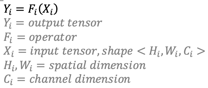
가장 기본이 되는 공식은 y=F(x)식이다.
여기서 x shape는 openCV에서 이미지 shape을 나타내는 단어인 height, width, channel을 의미한다.
한 모델에는 여러 레이어들이 쌓여있기 때문에 각 레이어를 지나면서 F(x)가 점점 많아진다.
수학적 용어로는 합성함수라고 하고 f5(f4(f3(f2(f1(x)))))로 표현하거나 f5◉f4◉f3◉f2◉f1(x)로 표현한다.
레이어의 갯수에 따라 f(x)의 갯수가 바뀌기 때문에 이 논문에서는 아래와 같이 표현했다.

<H, W, C> shape을 가진 X를 함수 F에 넣는데 함수 F는 한번의 i 안에서 nerwork length인 L만큼 계산을 반복한다. i가 s개까지 있으니 F(x)는 L만큼 반복하는 작업을 s번 수행하게 된다.
대부분의 ConvNet 디자인이 가장 best한 구조를 가지는 Fi를 찾는 것과 달리, model scaling은 미리 정의된 layer구조인 Fi를 변경하지 않고 length(Li), width(Ci), resolution(Hi, Wi)를 확장시키는 방법이다.

위에서 정의한 모델 N에 input의 depth(d), width(w), resolution(r)을 동시에 조절하여 가장 정확도가 높은 모델을 이루는 d, w, r의 관계를 찾는것이 목표다.
Scaling Dimensions

Depth(d)
- ConvNet에서 가장 일반적으로 사용하는 scaling
- 깊은 모델에서는 vanishing gradient 문제로 학습 어려움
- skip connection, batch normalization 방법이 해결책이 될 수 있지만 매우 깊은 모델에서는 효과 없음
(ex. ResNet-1000은 ResNet-101보다 훨씬 많은 layer를 가지고 있지만 비슷한 accuracy를 가짐) - Figure 3의 가운데 그래프를 보면 depth=8의 경우 accuracy가 오히려 떨어지는 것을 볼 수 있음
Width(w)
- width를 조절하는 것은 주로 작은 모델에서 사용
- wider network는 학습 과정에서 세밀한 특징을 잘 잡아내는 경향이 있음
- 하지만 극단적으로 넓지만 얕은 모델은 더 높은 수준의 특징을 포착하기 어려움
- Figure 3의 제일 왼쪽 그래프를 보면 width가 3.8에서 5.0으로 증가했음에도 accuracy는 큰 차이 없는 것을 볼 수 있음
Resolution(r)
- 고해상도 이미지일수록 세밀한 패턴을 잘 잡아냄
- 초기에는 224*224를 사용했지만 최근에는 600*600을 사용하는 모델도 있음
- Figure 3의 제일 오른쪽 그래프를 보면 width와 비슷하게 어느순간부터는 accuracy의 큰 상승 없이 FLOPS만 늘어나는 것을 볼 수 있음
Compound Scaling

그동안 경험적으로 각각의 차원(w, d, r)이 독립적이지 않다는 것을 알지만 최적의 경우를 찾아내기 위해서는 많은 시간이 소요되어 임의로 하나의 차원만 scaling하여 사용해왔다. Figure 4를 보면 4번의 실험을 통해 w, d, r를 모두 조절하여 accuracy가 어떻게 변화하는지를 나타냈다.
위 내용을 통해 아래 두가지 관찰(observation)을 확인할 수 있다.
Observation1
네트워크의 width, depth, resolution을 확장하면 accuracy가 향상되지만 더 큰 모델에서는 accuracy 상승률이 감소한다.
Obsercation2
더 나은 정확도와 효율성을 위해서 ConvNet scaling을 할 때 width, depth, resolution의 균형을 맞추는것이 매우 중요하다.

위 계산식에서 파이는 사용자의 리소스에 맞게 임의의 숫자를 넣어주면 된다.
알파, 베타, 감마는 앞으로 최적의 값을 찾아야하는 변수들이다.
- depth 2배 : FLOPS 2배
- width 2배 : FLOPS 4배 - width는 총 2번 연산이 되기 때문 (출력레이어, 다음 입력 레이어)
- resolution 2배 : FLOPS 4배 - resolution은 이미지의 가로x세로를 의미하기 때문에 가로2배, 세로2배로 총 4배가 됨
이 논문에서는 계산식 3번에 나온 것 처럼 알파*베타제곱*감마제곱의 값을 2로 제한했다.
그러므로 총 FLOPS는 2의 파이제곱만큼씩 커지게 된다.
EfficientNet Architecture
model scaling은 baseline network의 layer operator인 Fi를 바꾸지 않기 때문에 좋은 baseline network를 가지는 것은 매우 중요하다. 기존 ConvNet을 사용하여 scaling을 평가하는 방법에 더해 정확도와 FLOPS를 모두 최적화하는 EfficientNet을 개발했다. 여기서 EfficientNet은 더 큰 FLOPS 목표를 가진다는 점만 빼면 Mnas-Net과 유사한 아키텍처를 가진다.
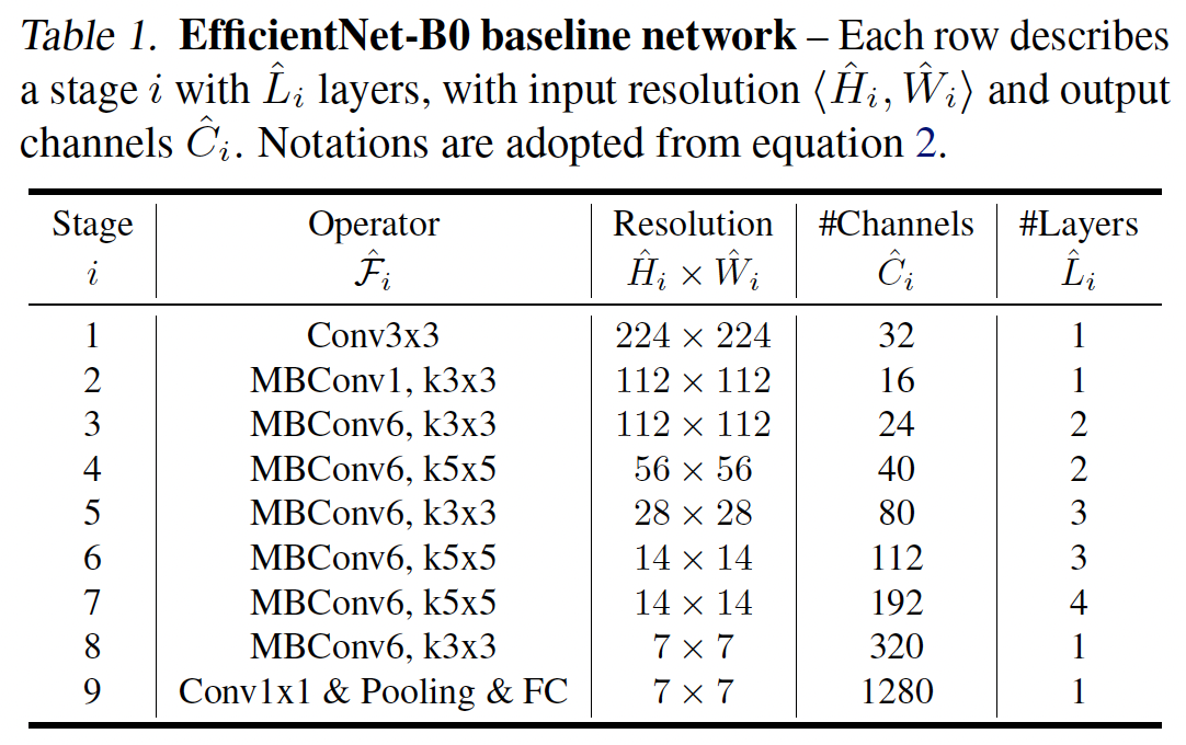
위 테이블을 보면 EfficientNet은 MBConv block을 이용하고(MnasNet에서 사용하는 Conv block임) 거기에 squeeze and excitation 최적화를 진행한다. squeeze and excitation은 논문(SENet; Squeeze and Excitation Networks)에서 제안한 개념으로 채널간의 가중치를 계산하여 성능을 높이는 방법이다.
최적화를 진행할 때 대형 모델의 경우, 알파, 베타, 감마의 값을 직접 설정하면 더 좋은 성능을 얻을 수 있지만 많은 비용이 들어가기 때문에 아래와 같이 작은 baseline network 에서 알파, 베타, 감마 값을 계산한 다음(STEP1), 다른 모든 모델에 대해 동일한 스케일링 계수를 사용한다(STEP2).
STEP1
- 사용 가능한 자원이 두배 더 많다고 가정하고 파이=1로 고정
- 계산식 2, 3번에 따라 알파, 베타, 감마에 대해서 small grid search를 수행
- 계산식 3번의 s.t. 조건에 의해 알파*베타제곱*감마제곱=2 제약 하에서 알파=1.2, 베타=1.1, 감마=1.15일 때 최상의 값을 가짐
STEP2
- 알파, 베타, 감마를 상수로 고정
- 계산식 3번에 따라 서로다른 파이를 설정하여 baseline network를 scaling
Experiments
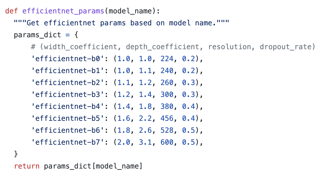
저자의 코드를 살펴보면 B0부터 B7까지 모델은 아래와 같이 width, depth, resolution, dropout_rate를 설정해주었다.
이 논문에서 제안한 compound scaling에 대해서 기존 ConvNet과 ErricientNet 적용 결과를 아래에서 확인할 수 있다.
비슷한 Accuracy를 보이는 기존모델과 EfficientNet을 비교했다. 표에서 확인할 수 있듯이 EfficientNet은 더 적은 Parameters를 가지고 더 적은 FLOPs를 수행했지만 더 좋은 Accuracy를 보인다.

Scaling Up MobileNets and ResNets

기존의 MobileNet과 ResNet에 compound scale을 적용했을 때 FLOPS와 Accuracy 차이를 보여준다.
compound scale을 적용한 모델이 더 좋은 성능을 보였다.
ImageNet Results for EfficientNet
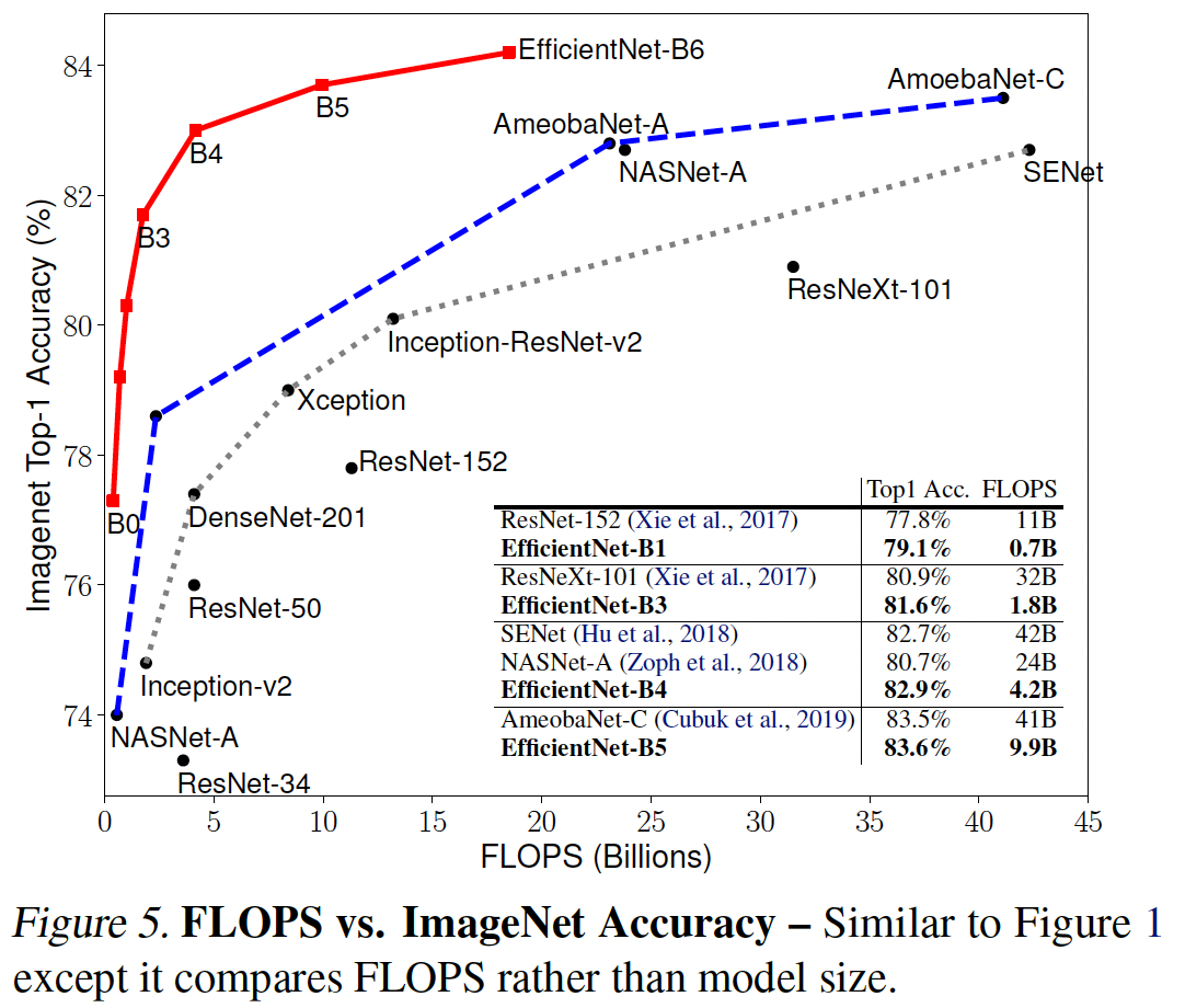
Figure 1 하고 비슷한 그래프처럼 보이지만 Figure 5에서는 X축이 파라미터 개수가 아니라 FLOPS를 나타낸다.
EfficientNet이 파라미터 수가 작으니까 FLOPs도 작게 나타나지만 Accuracy는 월등히 높은것을 확인할 수 있다.
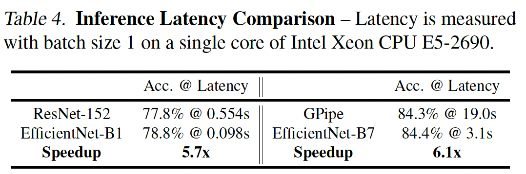
EfficientNet은 기존 ConvNet 보다 Params는 최대 8배 차이나거나 FLOPs가 최대 19배까지도 차이나지만 추론속도는 약 6배정도 빨라졌다. 속도 향상에도 긍정적인 효과가 있음을 알 수 있다.
Transfer Learning Results for EfficientNet
일반적으로 사용되는 전이학습 데이터셋을 가지고 EfficientNet을 평가한 결과는 아래와 같다.
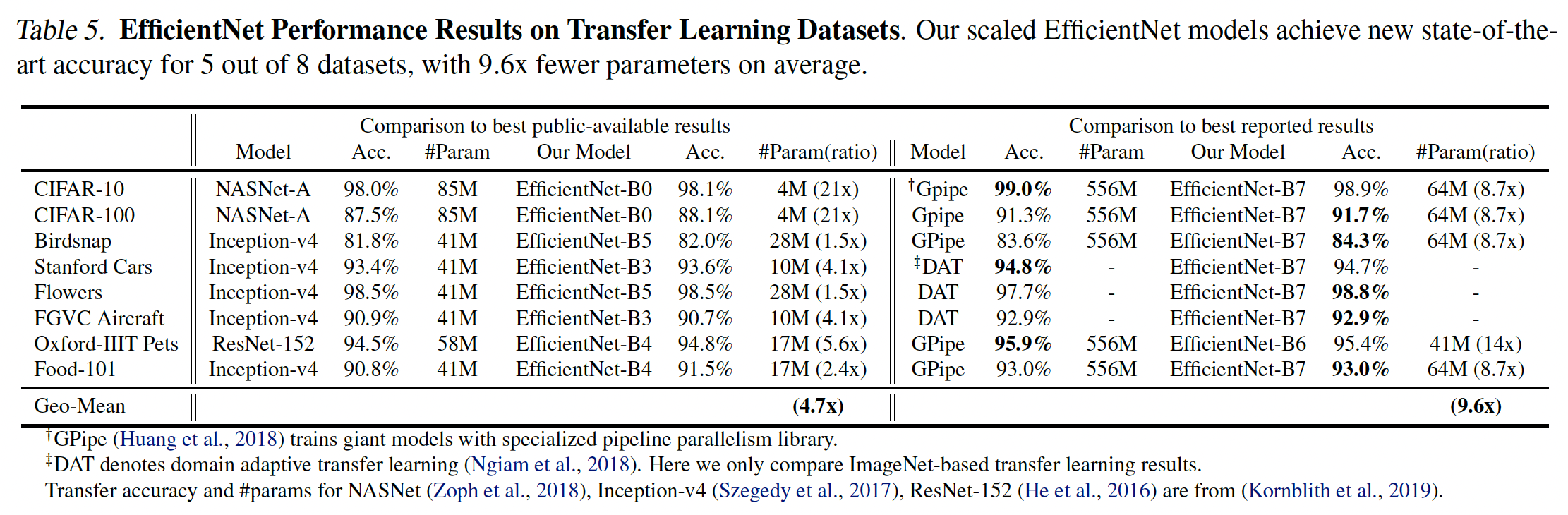
Tabel 5의 왼쪽(Comparison to best public-available results)은 NASNet이나 Inception-v4와 같이 공개된 모델들과 비교했을 때 EfficientNet 모델은 평균적으로 4.7배정도 적은 파라미터를 가지고 더 나은 정확도를 달성했음을 보여준다.
Tabel 5의 오른쪽(Comparison to best reported results)는 DATrhk GPipe를 포함한 최신 모델과 비교했을 때 EfficientNet 모델은 평균적으로 9.6배 정도 적은 파라미터를 가지고 더 나은 정확도를 달성했음을 보여준다. 이 부분은 Figure 6으로도 확인할 수 있지만 본 포스팅에서는 따로 그림을 삽입하지 않았다.
Discussion
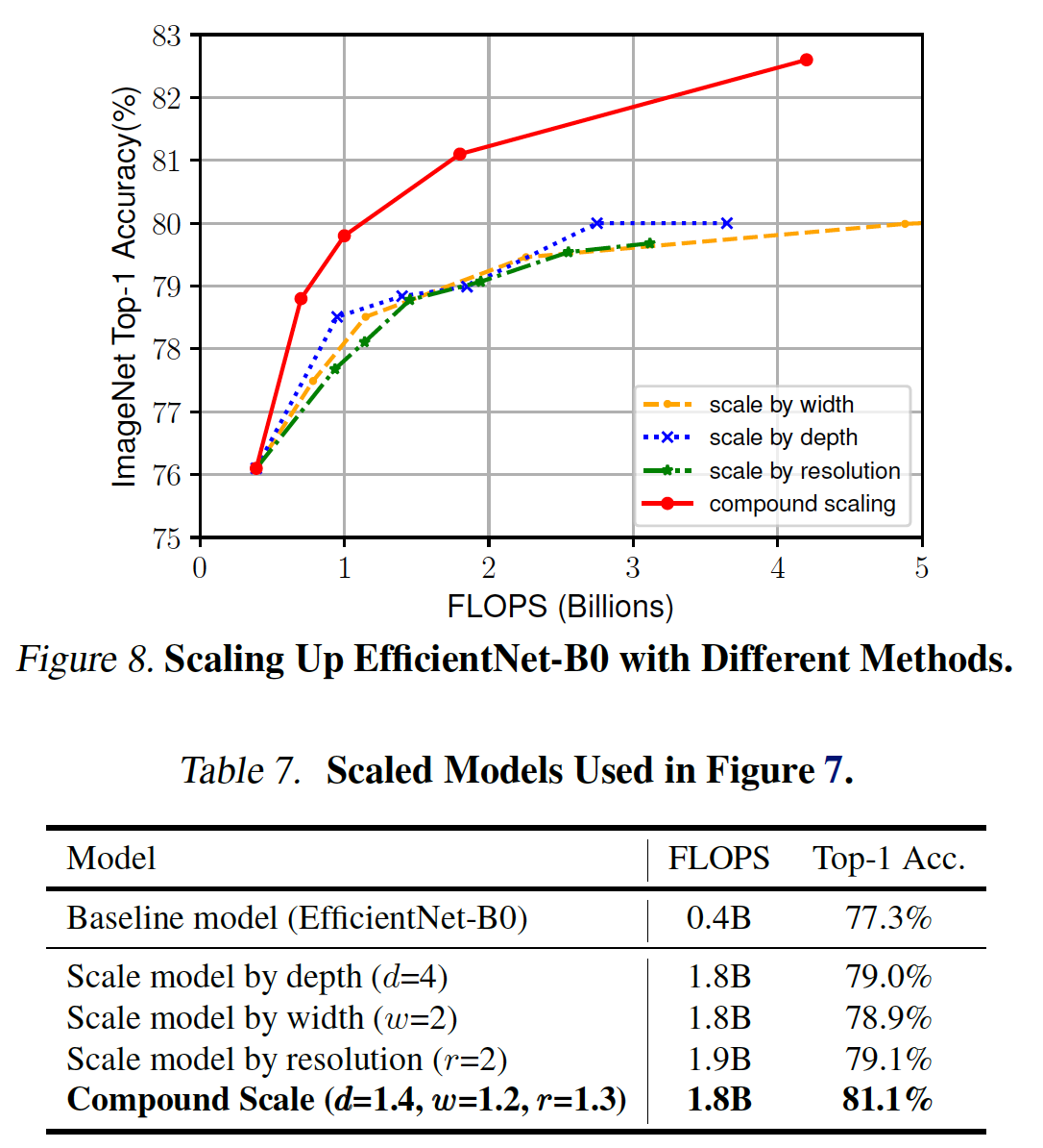
Figure 8에서 볼 수 있듯이 동일한 모델 EfficientNet-B0에 대하여 width scaling만 하는 경우, depth scaling만 하는 경우, resolution scaling만 하는 경우, compound scaling을 하는 경우에 compound scaling을 수행했을 때 가장 좋은 Accuracy를 보여준다.
Table 7에서는 비슷한 연산량을 가지는 경우(FLOPS가 1.8~1.9B), compound scaling을 하는 경우 Accuracy가 더 좋음을 보여준다.
Conclusion
이 논문에서는 ConvNet scaling을 체계적으로 연구하고 width, depth, resolution 값을 섬세하게 균형맞추어야 하지만 그동안은 그러지 못하여 더 나은 정확도와 효율성을 얻지 못했다는 것을 확인했다.
더 좋은 성능을 가지는 모델을 얻기 위해 compound scaling과 EfficientNet을 제안한다.
compound scaling을 적용한 EfficientNet은 더 적은 parameters와 FLOPs로 더 좋은 성능을 보였다.
논문리뷰
저자가 뭘 해내고 싶어했는가?
- 모델 성능을 높일 때 수동으로 조절했던 depth, width, resolution 사이의 관계을 수식으로 정리하여 한번에 스케일링하는 compound scaling을 제안, 더 짧은시간에 더 좋은 성능을 내는 모델을 만들고자 함
- compound scaling을 적용한 EfficientNet을 제안하여 효율성을 높인 모델 구축
이 연구의 접근에서 중요한 요소는 무엇인가?
기존에는 모델 성능 향상을 위해 width, depth, resolution 중 하나만 scaling했었는데 세가지 요소의 관계를 파악하여 수식으로 정의하고 세가지 요소를 모두 scaling 해보자!
논문을 보고 느낀점?
원래 수동으로 하나씩 설정해주는게 정말 귀찮은 일이라서 모든것을 설정하면 좋다는 것을 알지만 안하는 사람들이 많은데 이 논문을 발표한 사람들은 그 많은 수동설정을 하고, 하나씩 비교했다는 점에서 열정과 오기를 보았다.
어떤 프로젝트에 적용할 수 있는가?
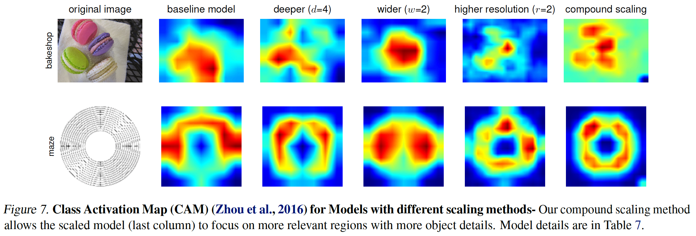
Figure 7을 보면 뭉텅이로 있는 이미지, 경계선이 모호한 이미지 등에 사용할 수 있을 것 같다.
이외에도 대부분의 경우 EfficientNet이 좋은 성능을 보일 것 같다.
추가적으로 공부해야할 것 또는 참고하고 싶은 다른 레퍼런스에는 어떤 것이 있는가?
- 비록 ResNet과 EfficientNet만 공부했을 뿐인데 이미지 데이터를 다루는 모델에 대한 이해도가 깊어진 것 같다.
- Object Detection에 EfficientNet을 적용한 EfficientDet도 있던데 한번 보면 좋을 것 같다.
- 추가적으로 Multi Modal을 공부하여 이미지+다른 데이터를 이용하는 모델도 공부하면 좋을 것 같다.
코드 구현
코드를 구현하기에 앞서 모델을 어떻게 build할지 아래 B0모델 구조와 논문저자의 코드를 참고했다.
B0 모델의 width=1, depth=1, resolution=224, dropout=0.2
resolution이 224이기 때문에 input shape 역시 224*224가 된다.
MBConv1, MBConv6의 숫자로 인해 expand를 1 또는 6으로 설정해야함을 알 수 있다.
또한 논문 내에는 Activation Function으로 SiLU(Swish)를 사용했다고 한다.
각 stage를 넘어갈 때 resolution값이 유지되면 stride=1, 그 값이 감소하면 감소하는 배수값이 stride 값이 된다.
예를들어 stage 3에서 stage 4로 넘어갈 때 resolution 값이 112*112에서 56*56으로 1/2배 줄어들었다. 따라서 이 때 stride=2다.
# import
import math
import torch
import torch.nn as nn
import torch.nn.functional as F

import os
from torchsummary import summary
from torch import optim
import torchvision
import torchvision.transforms as transforms
SE Block
Squeeze and Excitation은 위에서 언급했듯이 H * W * C 로 이루어져 있는 것을 1 * 1 * C로 펴준 다음에 다시 H * W * C 로 바꿔주면서 각 채널마다 가중치를 추가해준다.
# 논문에서 정한 reduction_ratio=0.25

class SEBlock(nn.Module):
    def __init__(self, in_channels, r=0.25):
        super().__init__()

        # se_channels : reduce layer out channels 계산
        se_channels = max(1, int(in_channels*r))

        self.se = nn.Sequential(# squeeze
                                nn.AdaptiveAvgPool2d(1),
                                # excitation
                                nn.Conv2d(in_channels, se_channels, kernel_size=1),
                                nn.SiLU(),
                                nn.Conv2d(se_channels, in_channels, kernel_size=1),
                                nn.Sigmoid()
                               )

    def forward(self, x):
        return x * self.se(x)
MBConv Block
MobileNetv2 개념을 대부분 가져와서 만들어진 블록이다.
MobileNet은 4단계로 이루어진다.
- stage1. Expantion
- stage2. Depth-wise Convolution
- stage3. Point-wise Convolution
- stage4. Skip Connection
Efficientnet에서 사용한 MBConvBlock은 3가지 차이점이 있다.
- 활성화함수 LeRU6대신 SiLU를 사용
- Depth-wise와 Point-wise 사이에 SE를 수행
- Depth-wise 수행 시 kernel_size를 3 또는 5로 사용
따라서 Efficientnet에 들어가는 MBConvBlock은 5단계로 이루어진다.
- stage1. Expantion
- stage2. Depth-wise Convolution
- stage3. Squeeze and Excitation (SEBlock)
- stage4. Point-wise Convolution
- stage5. Skip Connection
class MBConvBlock(nn.Module):
    def __init__(self, in_channels, out_channels, expand, kernel_size, stride=1, r=0.25, dropout_rate=0.2, bias=True):
        super().__init__()

        # 변수 설정
        self.dropout_rate = dropout_rate
        self.expand = expand

        # skip connection 사용을 위한 조건 지정
        self.use_residual = in_channels == out_channels and stride == 1

        # 논문에서 수행한 BatchNorm, SiLU 적용
        # stage1. Expansion
        expand_channels = in_channels*expand
        self.expansion = nn.Sequential(nn.Conv2d(in_channels, expand_channels, 1, bias=False),
                                       nn.BatchNorm2d(expand_channels, momentum=0.99),
                                       nn.SiLU(),
                                      )

        # stage2. Depth-wise convolution
        self.depth_wise = nn.Sequential(nn.Conv2d(expand_channels, expand_channels, kernel_size=kernel_size, stride=1, padding=1, groups=expand_channels),
                                        nn.BatchNorm2d(expand_channels, momentum=0.99),
                                        nn.SiLU(),
                                       )

        # stage3. Squeeze and Excitation
        self.se_block = SEBlock(expand_channels, r)

        # stage4. Point-wise convolution
        self.point_wise = nn.Sequential(nn.Conv2d(expand_channels, out_channels, 1, 1, bias=False),
                                        nn.BatchNorm2d(out_channels, momentum=0.99)
                                       )

    def forward(self, x):

        # stage1
        if self.expand != 1:
            x = self.expansion(x)

        # stage2
        x = self.depth_wise(x)

        # stage3
        x = self.se_block(x)

        # stage4
        x = self.point_wise(x)

        # stage5 skip connection
        res = x

        if self.use_residual:
            if self.training and (self.dropout_rate is not None):
                x = F.dropout2d(input=x, p=self.dropout_rate, training=self.training, inplace=True)

            x = x + res

        return x
EfficientNet 구축
사실 반복되는 구간은 for문으로 처리가 가능하지만 모델의 구조를 한눈에 파악할 수 있도록 각 layer를 모두 풀어서 작성했다.
class EfficientNet(nn.Module):
    def __init__(self, num_classes, width, depth, resolution, dropout):
        super().__init__()

        # stage1
        out_ch = int(32*width)
        self.stage1 = nn.Sequential(nn.Conv2d(in_channels=3, out_channels=out_ch, kernel_size=3, stride=2, padding=1),
                                    nn.BatchNorm2d(out_ch, momentum=0.99))

        # stage2
        self.stage2 = nn.Sequential(MBConvBlock(in_channels=out_ch, out_channels=16, expand=1, kernel_size=3, stride=1, dropout_rate=dropout))

        # stage3
        self.stage3 = nn.Sequential(MBConvBlock(in_channels=16, out_channels=24, expand=6, kernel_size=3, stride=2, dropout_rate=dropout),
                                    MBConvBlock(in_channels=24, out_channels=24, expand=6, kernel_size=3, stride=1, dropout_rate=dropout),
                                   )

        # stage4
        self.stage4 = nn.Sequential(MBConvBlock(in_channels=24, out_channels=40, expand=6, kernel_size=5, stride=2, dropout_rate=dropout),
                                    MBConvBlock(in_channels=40, out_channels=40, expand=6, kernel_size=5, stride=1, dropout_rate=dropout),
                                   )

        # stage5
        self.stage5 = nn.Sequential(MBConvBlock(in_channels=40, out_channels=80, expand=6, kernel_size=3, stride=2, dropout_rate=dropout),
                                    MBConvBlock(in_channels=80, out_channels=80, expand=6, kernel_size=3, stride=1, dropout_rate=dropout),
                                    MBConvBlock(in_channels=80, out_channels=80, expand=6, kernel_size=3, stride=1, dropout_rate=dropout),
                                   )

        # stage6
        self.stage6 = nn.Sequential(MBConvBlock(in_channels=80, out_channels=112, expand=6, kernel_size=5, stride=1, dropout_rate=dropout),
                                    MBConvBlock(in_channels=112, out_channels=112, expand=6, kernel_size=5, stride=1, dropout_rate=dropout),
                                    MBConvBlock(in_channels=112, out_channels=112, expand=6, kernel_size=5, stride=1, dropout_rate=dropout),
                                   )

        # stage7
        self.stage7 = nn.Sequential(MBConvBlock(in_channels=112, out_channels=192, expand=6, kernel_size=5, stride=2, dropout_rate=dropout),
                                    MBConvBlock(in_channels=192, out_channels=192, expand=6, kernel_size=5, stride=1, dropout_rate=dropout),
                                    MBConvBlock(in_channels=192, out_channels=192, expand=6, kernel_size=5, stride=1, dropout_rate=dropout),
                                    MBConvBlock(in_channels=192, out_channels=192, expand=6, kernel_size=5, stride=1, dropout_rate=dropout),
                                   )

        # stage8
        self.stage8 = nn.Sequential(MBConvBlock(in_channels=192, out_channels=320, expand=6, kernel_size=3, stride=1, dropout_rate=dropout))

        # stage9
        self.last_channels = math.ceil(1280*width)
        self.stage9 = nn.Conv2d(in_channels=320, out_channels=self.last_channels, kernel_size=1)

        # result
        self.out_layer = nn.Linear(self.last_channels, num_classes)

    def forward(self, x):
        x = self.stage1(x)
        x = self.stage2(x)
        x = self.stage3(x)
        x = self.stage4(x)
        x = self.stage5(x)
        x = self.stage6(x)
        x = self.stage7(x)
        x = self.stage8(x)
        x = self.stage9(x)
        x = F.adaptive_avg_pool2d(x, (1, 1)).view(-1, self.last_channels)
        x = self.out_layer(x)

        return x
# efficientnet 모델 b0 ~ b7
def efficientnet_b0(num_classes=10):
return EfficientNet2(num_classes=num_classes, width=1.0, depth=1.0, resolution=224, dropout=0.2)
def efficientnet_b1(num_classes=10):
return EfficientNet2(num_classes=num_classes, width=1.0, depth=1.1, resolution=240, dropout=0.2)
def efficientnet_b2(num_classes=10):
return EfficientNet2(num_classes=num_classes, width=1.1, depth=1.2, resolution=260, dropout=0.3)
def efficientnet_b3(num_classes=10):
return EfficientNet2(num_classes=num_classes, width=1.2, depth=1.4, resolution=300, dropout=0.3)
def efficientnet_b4(num_classes=10):
return EfficientNet2(num_classes=num_classes, width=1.4, depth=1.8, resolution=380, dropout=0.4)
def efficientnet_b5(num_classes=10):
return EfficientNet2(num_classes=num_classes, width=1.6, depth=2.2, resolution=456, dropout=0.4)
def efficientnet_b6(num_classes=10):
return EfficientNet2(num_classes=num_classes, width=1.8, depth=2.6, resolution=528, dropout=0.5)
def efficientnet_b7(num_classes=10):
return EfficientNet2(num_classes=num_classes, width=2.0, depth=3.1, resolution=600, dropout=0.5)
모델이 잘 구축되었는지 확인하기 위해서 임의의 텐서를 넣어서 결과와 파라미터 값을 확인했다.
if __name__ == '__main__':
    device = 'cuda' if torch.cuda.is_available() else 'cpu'

    x = torch.randn(4, 3, 224, 224).to(device)
    model = efficientnet_b0().to(device)
    output = model(x)
    print('output size:', output.size())

    summary(model, input_size=(3, 224, 224))
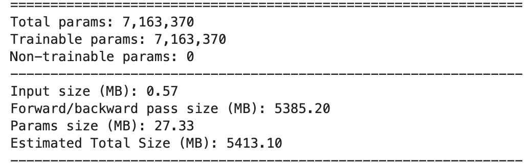
기존 파라미터는 약 500만개 정도 나오는데 716만개의 파라미터가 나왔으니 살짝 오버된 감이 있지만 그럭저럭 쓸만하지 않을까...
EfficientNet 실습
내가 만든 모델 쓸만하지 않을까 싶었는데 학습하는데 시간이 너무 오래 걸림....efficientnet인데 시간 오래걸리는게 맞나?
# 변수설정
batch_size = 128
n_epochs = 10
lr = 0.1
data_dir = '/data/cifa10
# 모델호출
# 위에서 내가 만든 모델 사용
model = EfficientNet(model_num='b0', num_classes=10)
# 모델 패키지 사용
from efficientnet_pytorch import EfficientNet
model = EfficientNet.from_pretrained('efficientnet-b0')
# 비용함수, 옵티마이저 정의
cost = nn.CrossEntropyLoss()
optimizer = torch.optim.Adam(model.parameters(), lr=lr)# 데이터 transform
transform = transforms.Compose([transforms.Resize((224, 224)),
transforms.ToTensor(),
transforms.Normalize(mean=[0.485, 0.456, 0.406], std=[0.229, 0.224, 0.225]),
])
# 데이터 불러오기
trainset = torchvision.datasets.CIFAR10(root=data_dir+'/train', train=True, download=True, transform=transform)
valset = torchvision.datasets.CIFAR10(root=data_dir+'/test', train=False, download=True, transform=transform)
# DataLoader
trainloader = torch.utils.data.DataLoader(trainset, batch_size=batch_size, shuffle=True, num_workers=2)
valloader = torch.utils.data.DataLoader(valset, batch_size=batch_size, shuffle=False, num_workers=2)# 학습
for epoch in range(n_epochs):
avg_cost = 0
accuracy = 0
for X, Y in trainloader:
X = X.to(device)
Y = Y.to(device)
# 가설
hypothesis = model(X)
# loss
loss = cost(hypothesis, Y)
# update
optimizer.zero_grad()
loss.backward()
optimizer.step()
# avg_cost
avg_cost += loss / len(trainloader)
correct = torch.argmax(hypothesis, 1) == Y
accuracy = correct.float().mean()
print(f'Epoch {epoch}/{n_epochs}\tLoss {avg_cost:.4f}\tAcc {accuracy:.4f}')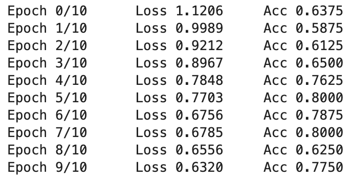
cuda를 썼는데도 생각보다 시간이 오래 걸려서 10번만 돌려봤다. 최고 Accuracy는 0.8이 나왔다.
pre-trained를 사용했을 때는 2epoch만에 94%가 나왔었는데 내가 빌드한 모델은 어딘가 부족한 것 같으면서도 다른 사람은 0.65가 나온걸 보면 괜찮은것 같기도....?
# test

avg_accuracy = []

for X, Y in valloader:
    X = X.to(device)
    Y = Y.to(device)

    pred = model(X)
    correct = torch.argmax(pred, 1) == Y
    accuracy = correct.float().mean()
    avg_accuracy.append(accuracy)

print('Accuracy:', sum(avg_accuracy)/len(avg_accuracy))
train 때 최고 정확도는 0.8이 나왔는데 test때 평균 정확도는 0.785가 나왔다.
정확도가 그리 높지는 않지만 잘 학습되었다는 것을 알 수 있다.
참고
<논문리뷰>
TensorFlowKR 논문읽기모임 - PR169 논문리뷰
AI꿈나무 - [논문읽기] EfficientNet(2019) 리뷰
lynnshin - [논문리뷰] EfficientNet정리 (MobileNet부터 EfficientNet까지)
<EfficientNet Pytorch 코드 구현>
논문저자 - EfficientNet Tensorflow 모델 구현 코드 github
zsef123 - EfficientNet Pytorch 모델 구현 코드 github
linksense - EfficientNet Pytorch 모델 구현 코드 github
<EfficientNet Pytorch 실습>
AI꿈나무 - [논문구현] Pytorch로 EfficientNet 구현하고 실습하기
EfficientNet-Pytorch library Qick Start
Present_Kim - EfficientNetB0 colab에서 pytorch로 구현해서 CIFAR-10 학습시켜보기